
To efficiently execute this stage of the project, reviewing the obtained
data types and identifying the extant data levels are conducive measures to infer the appropriate
exploration methods.
We began the preprocessing stage by resizing the collected organized data
and dropping the empty rows and negligible columns.
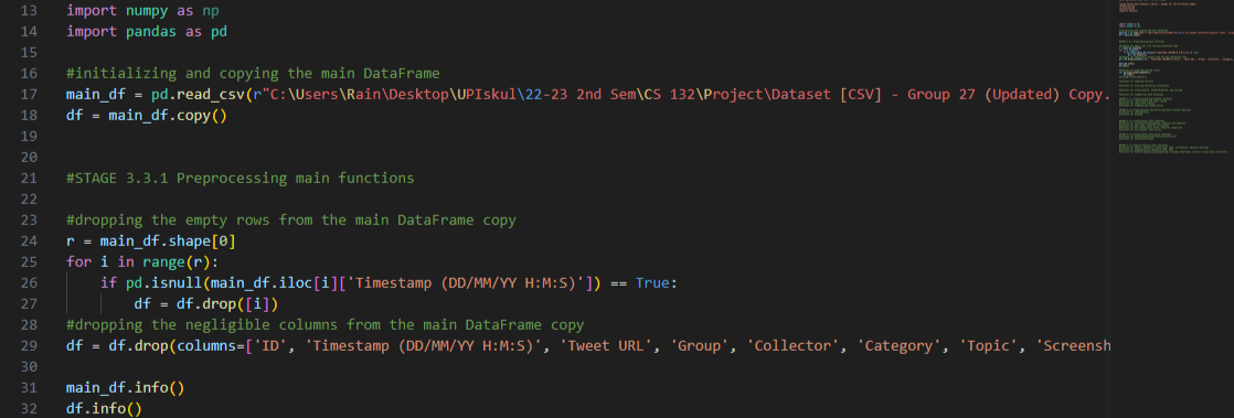
It was deduced that rows with empty values in the ‘Timestamp (DD/MM/YY H: M:S)’
column are consequently blank rows.
Additionally, the aforesaid columns included in the dropped list are:
[‘ID’, ‘Timestamp (DD/MM/YY H: M:S)’, ‘Tweet URL’, ‘Group’, ‘Collector’, ‘Category’, ‘Topic’,
‘Screenshot’, ‘Reviewer’, ‘Review’].
These columns were distinguished as negligible since their values were used to review or identify—not
classify—row entries. Thus, they do not have any bearing on the research question.
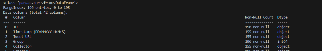
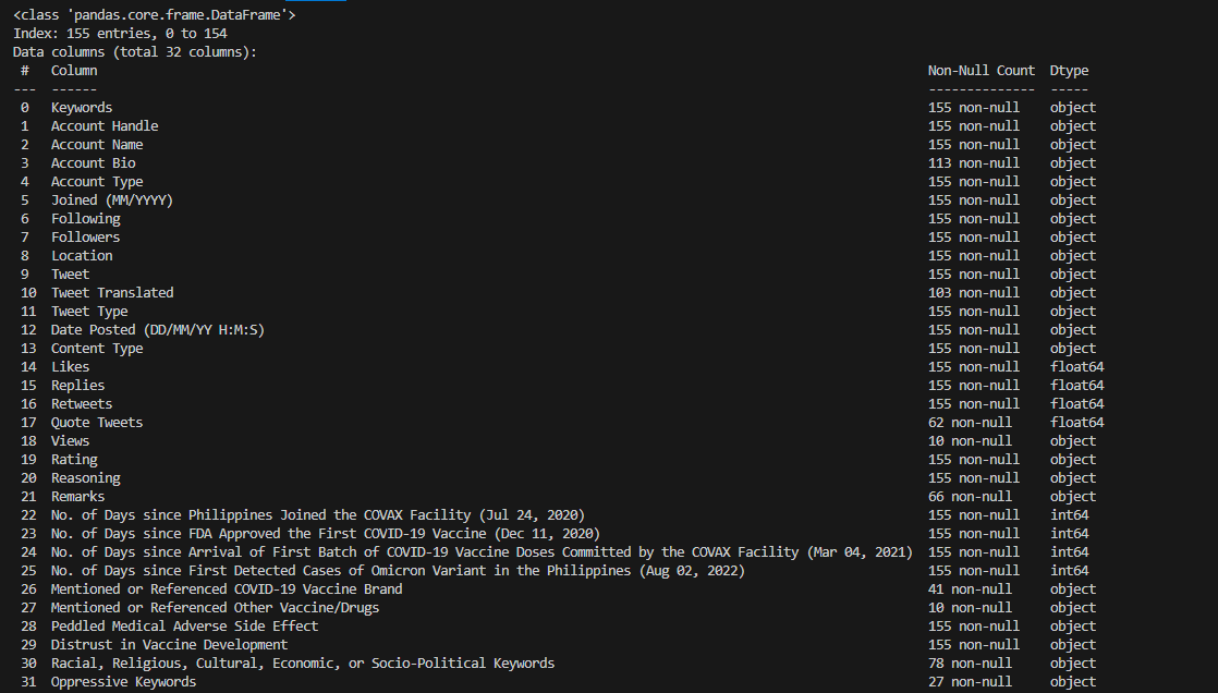
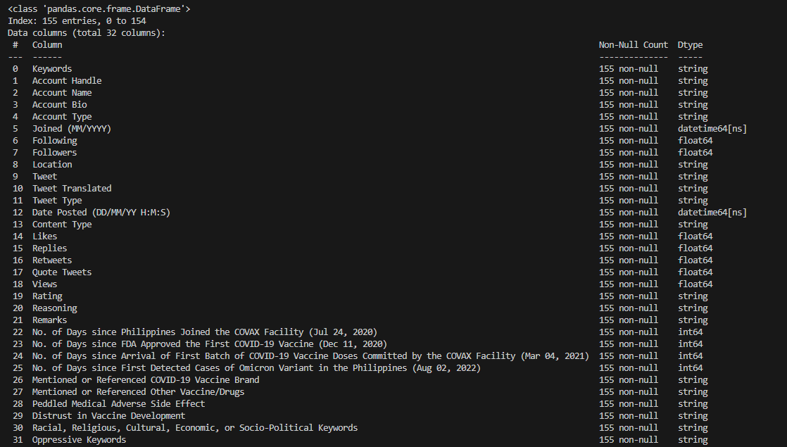
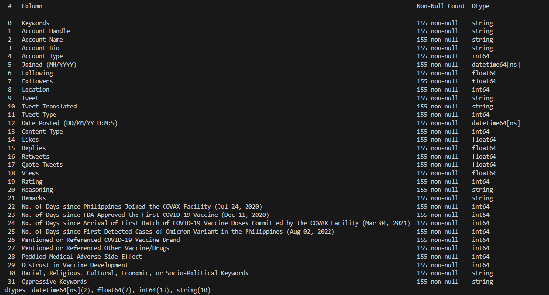
After this step, we arrived at a more refined structured
data that has 32 columns and 155 rows.
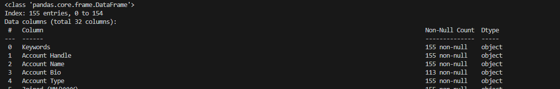
Of the remaining 32 columns, their respective types are as follows:
Qualitative Data – ['Keywords', 'Account Handle', 'Account Name',
'Account Bio', 'Account Type', 'Location', 'Tweet', 'Tweet Translated', 'Tweet Type', 'Content Type',
'Rating', 'Reasoning', 'Remarks', 'Mentioned or Referenced COVID-19 Vaccine Brand', 'Mentioned or Referenced
Other Vaccine/Drugs', 'Peddled Medical Adverse Side Effect', 'Distrust in Vaccine Development', 'Racial,
Religious, Cultural, Economic, or Socio-Political Keywords', 'Oppressive Keywords']
Quantitative Data (Discrete) – [ 'Joined (MM/YYYY)', 'Date Posted
(DD/MM/YY H:M:S)’, 'Following', ‘Followers’, 'Likes', 'Replies', 'Retweets', 'Quote Tweets', 'Views', 'No.
of Days since Philippines Joined the COVAX Facility (Jul 24, 2020)', 'No. of Days since FDA Approved the
First COVID-19 Vaccine (Dec 11, 2020)', 'No. of Days since Arrival of First Batch of COVID-19 Vaccine Doses
Committed by the COVAX Facility (Mar 04, 2021)', 'No. of Days since First Detected Cases of Omicron Variant
in the Philippines (Aug 02, 2022)']
Quantitative Data (Continuous) – [ ]
Additionally, the existing columns and their levels are classified into:
Nominal Level – ['Account Type', 'Location', 'Tweet Type', 'Content
Type', 'Rating', 'Mentioned or Referenced COVID-19 Vaccine Brand', 'Mentioned or Referenced Other
Vaccine/Drugs', 'Peddled Medical Adverse Side Effect', 'Distrust in Vaccine Development']
Ordinal Level –[]
Interval Level – ['Joined (MM/YYYY)', 'Date Posted (DD/MM/YY H:M:S)',
'No. of Days since Philippines Joined the COVAX Facility (Jul 24, 2020)', 'No. of Days since FDA Approved
the First COVID-19 Vaccine (Dec 11, 2020)', 'No. of Days since Arrival of First Batch of COVID-19 Vaccine
Doses Committed by the COVAX Facility (Mar 04, 2021)', 'No. of Days since First Detected Cases of Omicron
Variant in the Philippines (Aug 02, 2022)']
Notes: Pandas Timestamp and Python Datetime are interchangeable data
objects that represent dates in the form of integers.
The “No. of Days” indicated in the columns listed above may take negative values, which means they
occurred before a specified point in time. Since this could be the case, such measurements have no
starting zero and are intervals.
Ratio Level – ['Following', ‘Followers’, 'Likes', 'Replies',
'Retweets', 'Quote Tweets', 'Views']
Textual Data – ['Keywords', 'Account Handle', 'Account Name',
'Account Bio', 'Tweet', 'Tweet Translated', 'Reasoning', 'Remarks', 'Racial, Religious, Cultural, Economic,
or Socio-Political Keywords', 'Oppressive Keywords']
Using the Pandas DataFrame.info()
method, we were able to ensure the expected number of cells that have missing values.
As for detecting and handling the missing values, the function
missing_values_handler() was utilized:
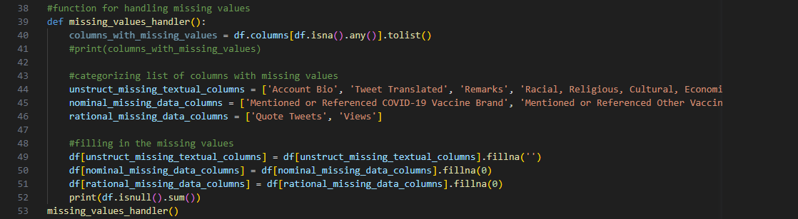
Line 40 initializes a list of columns that have missing values using
DataFrame.isna().any() method:
['Account Bio', 'Tweet Translated', 'Quote Tweets', 'Views', 'Remarks', 'Mentioned or Referenced
COVID-19 Vaccine Brand', 'Mentioned or Referenced Other Vaccine/Drugs', 'Racial, Religious, Cultural,
Economic, or Socio-Political Keywords', 'Oppressive Keywords'].
The values of columns 'Tweet Translated', ‘Quote Tweets’, and ‘Views’ are dependent on the entry tweet.
Expectedly, they may have empty values when there is no pertinent observation of a tweet’s characteristics.
Meanwhile, the rest of the columns in the list above are either optional or have inherent ‘None’ choices
and were classified as such during data collection.
Line 49 deals with the missing values of ‘Account Bio’, ‘Tweet Translated’, ‘Remarks’, 'Racial,
Religious, Cultural, Economic, or Socio-Political Keywords', and 'Oppressive Keywords' using replacement
with an arbitrary zero represented by an empty string.
This method was used because these columns contain unstructured textual data and will be further refined
later through natural language processing.
Line 50 handles the missing values of 'Mentioned or Referenced COVID-19 Vaccine Brand' and 'Mentioned or
Referenced Other Vaccine/Drugs' using replacement with an arbitrary zero represented by an integer.
On
the other hand, this approach was applied for these columns given that they contain nominal data and will be
encoded later into numerical values.
Line 51, for thoroughness, applies the same technique as Line 50 to the columns ‘Quote Tweets’ and
‘Views’, which are members of the ratio data level.
While these tweet characteristics are represented as
numerical counts, the replacement with the mean method was not applied to avoid introducing bias since these
are optional fields.
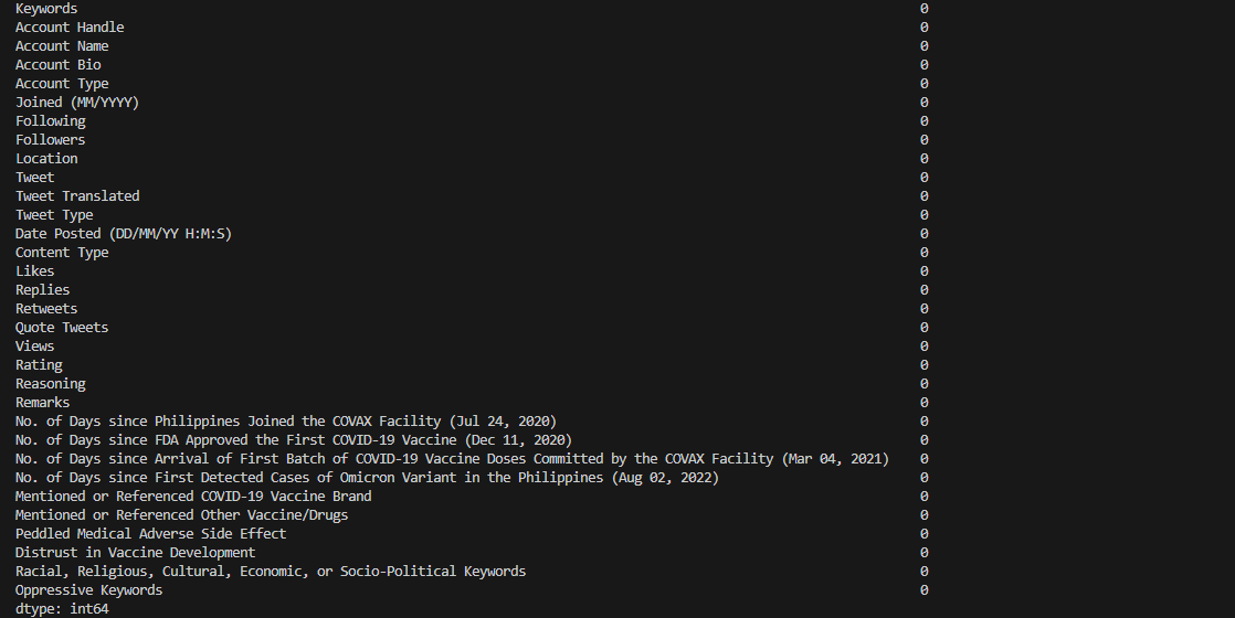
Finally, the total number of missing values in each column can be
summarized and confirmed using the output of the method df.isnull().sum().
Following the imputation steps, it is noticeable using info() method that there are discrepancies with the data types of the
columns.
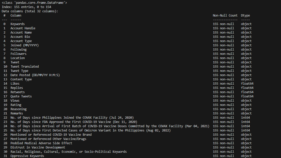
Many columns have object
dtype, meaning these columns might contain strings or mixed types of data. Furthermore, some
columns are expected to contain numerical values and have object dtype instead.
This needs to be resolved first before treating possible outliers because the values must be uniform for
statistical operations to be applicable.
The function formatting_handler() was used to address formatting inconsistencies in
the data:
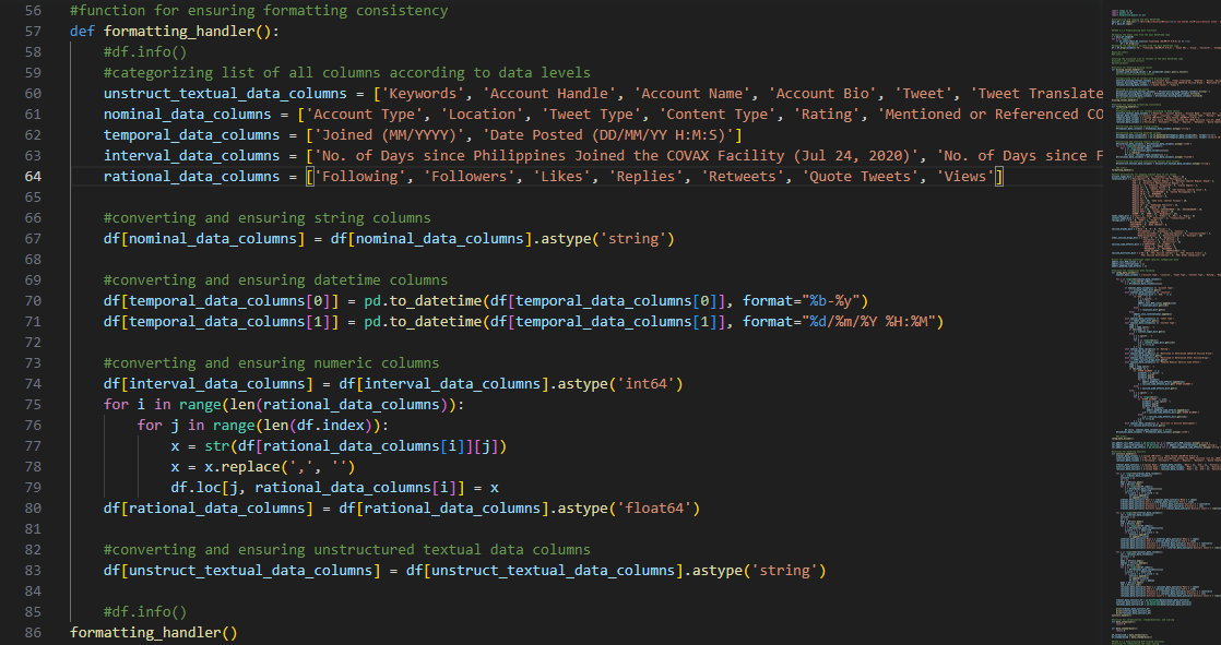
Lines 59-63 initialize lists that group all columns into their
appropriate data level classification.
Lines 66-79 then transmute the non-conforming values accordingly. The following conditions were
prioritized for this method:
As recommended by Pandas documentation, StringDtype is preferred over object
dtype because the latter can accidentally store non-strings. Thus, instances of object dtype columns that strictly contain string literals were
transformed.
Records of date and timestamps were initially relegated also as object
dtype and were thus changed to DatetimeTZ dtype.
Columns that have object dtype and must be comprised of numerical integer values, though already
compliant, were still converted to int64 data type as a
precaution.
Columns that must contain numerical float values, meanwhile, were stripped of comma separators before
converting to float64 data type.
Line 82 handles the remaining columns of unstructured textual data by
transforming them into StringDtype for later language processing.
Finally, info()
method was used again to check that the appropriate data types for all columns and date formatting
requirements were satisfied.
As fulfilled in the previous preprocessing steps, we were able to
identify which columns contain nominal data and would therefore require categorical encoding:
['Account Type', 'Location', 'Tweet Type', 'Content Type', 'Rating', 'Mentioned or Referenced COVID-19
Vaccine Brand', 'Mentioned or Referenced Other Vaccine/Drugs', 'Peddled Medical Adverse Side Effect',
'Distrust in Vaccine Development']
Global Python dictionaries were first initialized for data encoding and later decoding during the
analysis stage.
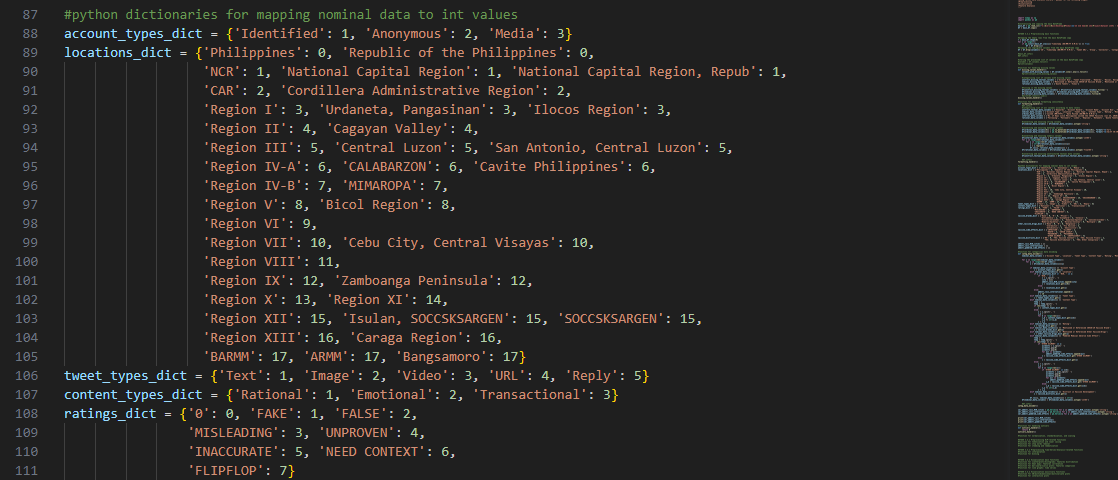
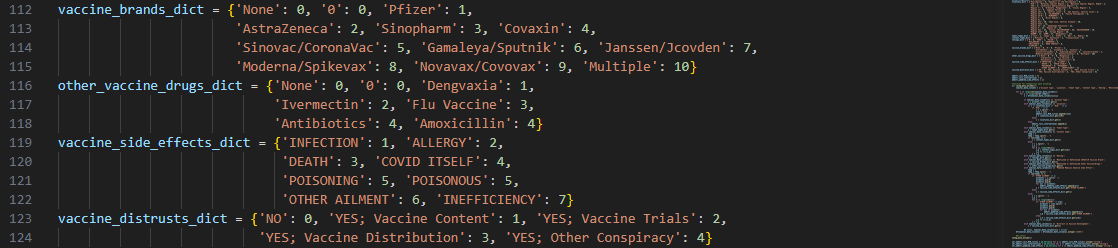
Apart from dictionaries, empty lists were also created as ‘catch basins’ for optional subcategories included in the categorical data. These will be transformed into Series dtype for analysis afterward.

The function categ_data_encoder()
assigns integer values to the categorical data using the appropriate dictionary:
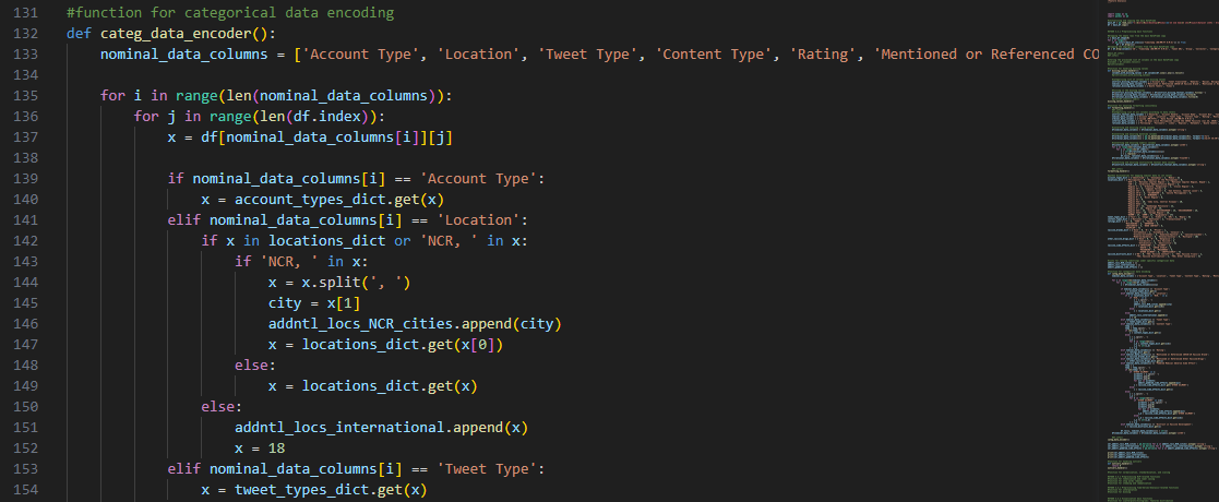
A for-loop that iterates over the columns with nominal data and
accesses their values was the main approach used for this step of numerical encoding.
Since dictionaries were already made available for mapping the categories, get() method allowed us to obtain the corresponding integer values.
Some columns required additional string manipulation to extract the data, like the ‘Location’
characteristic, because it contains an optional substring field for ‘city name’ that cannot be explicitly
integrated into category labels.
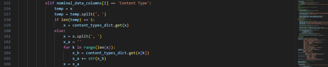
As for columns that may have more than one category, such as the
‘Content Type’, we used string concatenation to represent a sequence of one-digit integer values, each
corresponding to a label.
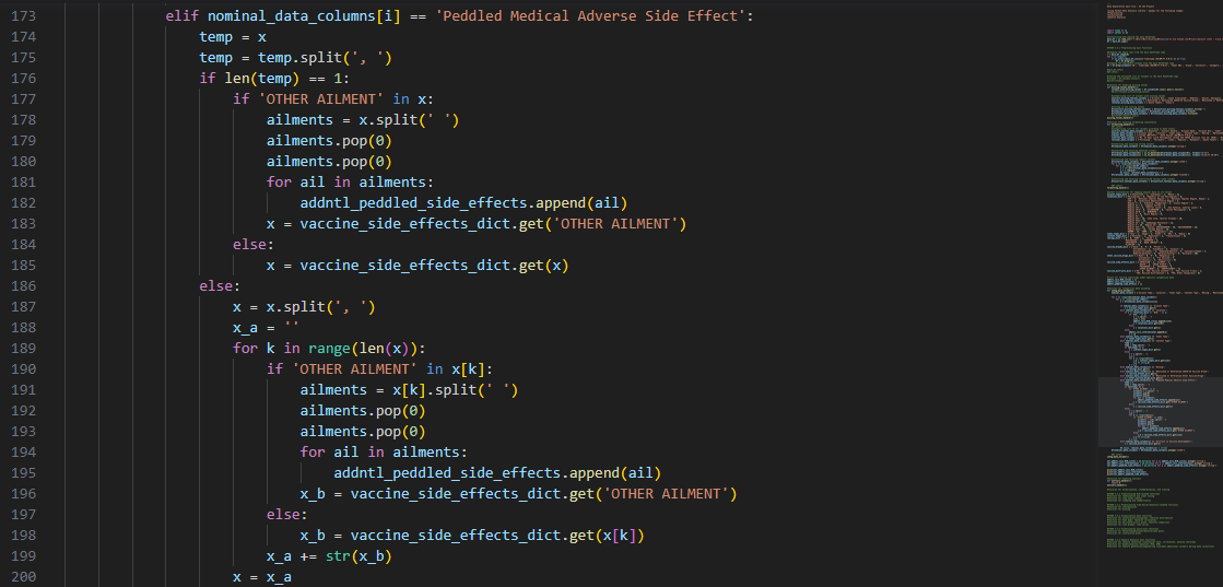
Lastly, for nominal columns that might contain more than two
subcategories e.g., 'Peddled Medical Adverse Side Effect', we handled the encoding by passing conditional
statements and manipulating the obtained sublists.
Since we only stored the primary category labels, we used the empty lists that were instantiated
earlier. After converting to Series dtype, we can use the textual
data as variables of natural language processing and other steps later.
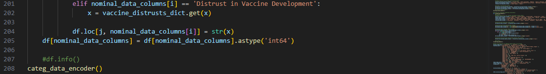
Upon completing this step, we also ensured that the data types of the
columns are numerical in the form of int64. It can also be confirmed
using
info
() method that the data types were no longer strings literals.
To detect outliers, we adhered to the computation of z-scores and
identifying data points that have greater than +3 or less than -3 z-scores.
With the aid of the function outliers_handler(), separate
dataframes for columns pertinent to temporal data, interval data, and rational data were created to store
characteristics about outlier data itself
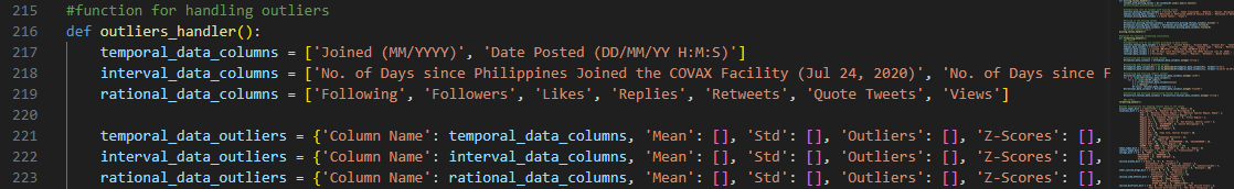
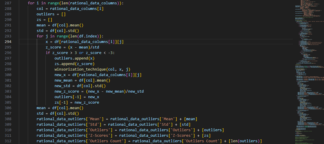
Moving forward, for-loops that iterate through the data features
serve as the primary tool for obtaining the necessary statistical values.
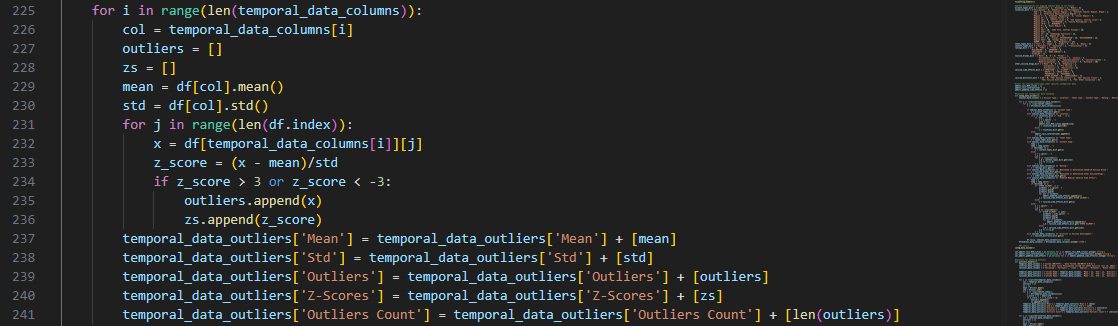
The function calculates the mean and standard deviation, which are
used to calculate individual z-scores to be compared.
It then adds the verified outliers and their z-scores to a list for the current column and is repeated
for each characteristic that contain temporal data.
These steps were also applied to the other groups of data level—interval and rational—and the results
were stored in separate dictionaries.
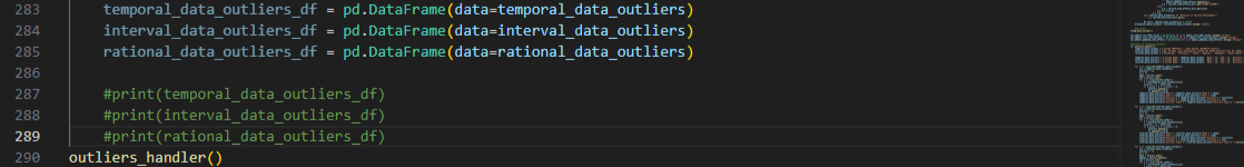
Once the function is done processing, it creates a DataFrame dtype from the dictionaries using the built-in pandas utility.
We used print() as a straightforward method to check the obtained
outliers.
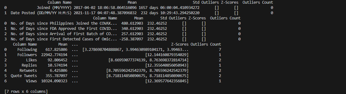
From the output, no outliers were detected in any of the columns
under the groups of temporal and interval data. As for rational data, we found 1 to 2 outliers with
significantly higher z-scores in most of the columns. Additionally, there were 7 outliers in the ‘Following’
column.
We deduced that they are heavily skewing the mean and standard deviation. However, we also concluded
that they are not representative of the whe whole data.
Most of the detected outliers are unique
individual cases dependent on the Twitter account owner i.e., the tweet was posted by an account that has a
lot of influence (followers/following counts).
As a solution, the method of winsorization to a fixed percentile was applied. We opted not to drop the
rows because our research question puts more emphasis on the context of the tweets, not on the account who
posted them.
The for-loops that iterate through the columns were subsequently modified to execute the adjustments to
the outlier values:
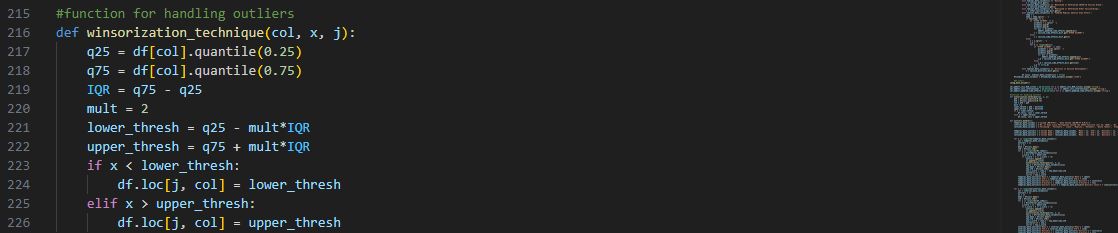
The auxiliary function winsorization_technique() defines a lower and
upper threshold for the dataset based on the 25th and 75th percentiles.
A multiplier is chosen—2 represents the smallest 2% and largest 2% of values—and is multiplied to the
Interquartile Range that represents the spread of the dataset.
Outliers that are below the lower threshold are replaced with the 25th percentile minus the multiplier
times the IQR. As for outliers above the upper threshold, they are replaced with the 75th percentile plus
the multiplier times the IQR.
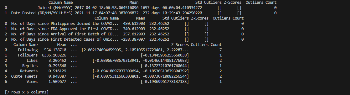
Upon executing the modified program, we observed that there are
significant differences between the mean and standard deviation values of the old output with the new
output.
The z-scores of the recorded outliers were also recomputed and can be confirmed that they are now within
the acceptable range.
In preparation for the machine learning steps, we applied four
scaling methods to our dataset using iterative programming techniques and some of Python’s computational
libraries. To emphasize, these methods were only applied to data features that have inherent numeric values.
We started off with data_min_max_scaler() function, or more
commonly-known as normalization:
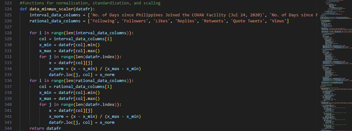
It takes the minimum and maximum values in a specific data feature
and utilizes these to scale the data point to a range between 0 and 1.
To get the normalized value of x, the minimum values is subtracted from it and the result is divided by
the range, or the difference between the maximum and minimum values.
Following normalization, we also implement z-score normalization or
standardization using the function, data_standardizer():
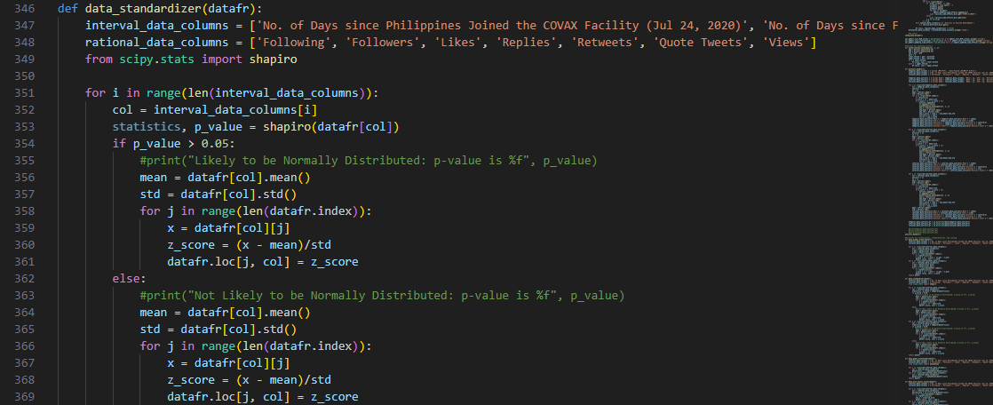
The z-score computation was already explained in previous sections.
But another key detail to standardization is that it assume a normally distributed dataset.
To ascertain this prerequisite, we used the Shapiro-Wilk test using the shapiro function from SciPy,
which then returns a p-value corresponding to a significance level from normality.
Upon running the program, we found that our dataset is not normally distributed for the features in the
interval_data_columns and rational_data_columns.
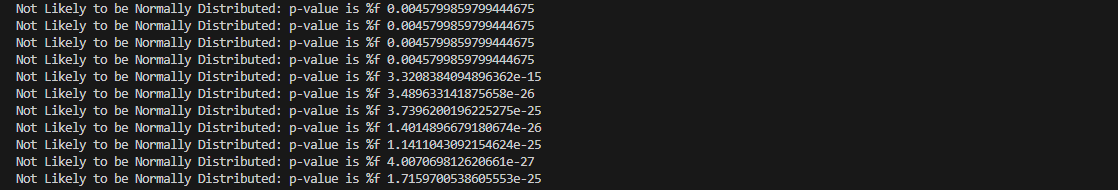
For comprehensiveness, however, we still opted to standardize our
dataset as a future reference.
Given that we our dataset is not leaning towards normal distribution, we decided
to apply power transformation to address possible skewness or th heavy tails using data_power_transformer():
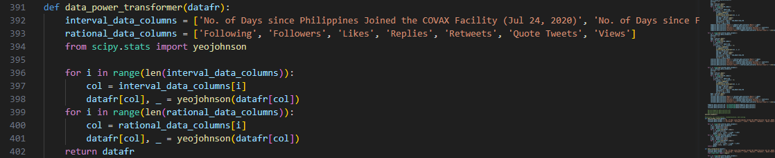
The Yeo-Johnson power transformation, as pulled also from Python
SciPy library, uses a lambda parameter to scale the data points.
We also chose this method because it can handle both positive and negative values that are present in
our dataset, unlike its curtailed version—Box-Cox method.
Lastly, data_unit_vector_scaler() is a
function that scales the characteristics of our dataset to have a consistent magnitude of 1. We concluded
that this additional step will be useful later for feature analysis.
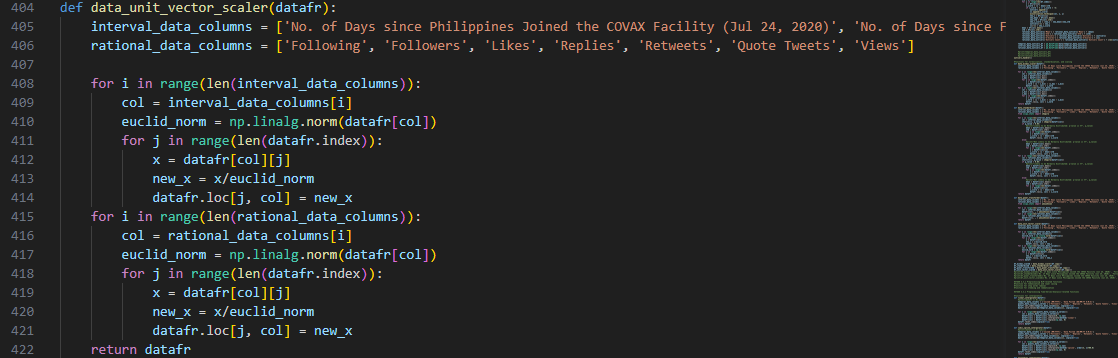
Unlike min-max scaling, this approach normalizes the magnitude of
vectors using the Euclidian norm, computed through the aid of NumPy’s built-in method.
The four functions that were introduced above were implemented to transform four
copies of the original dataframe.
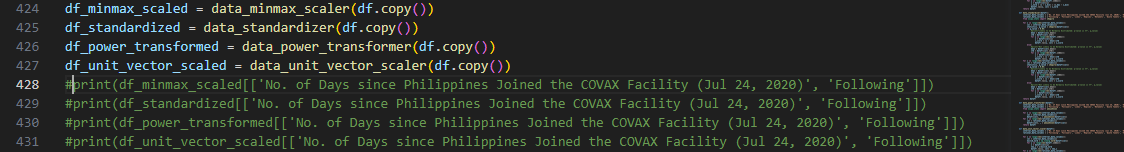
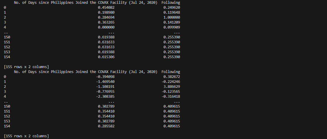
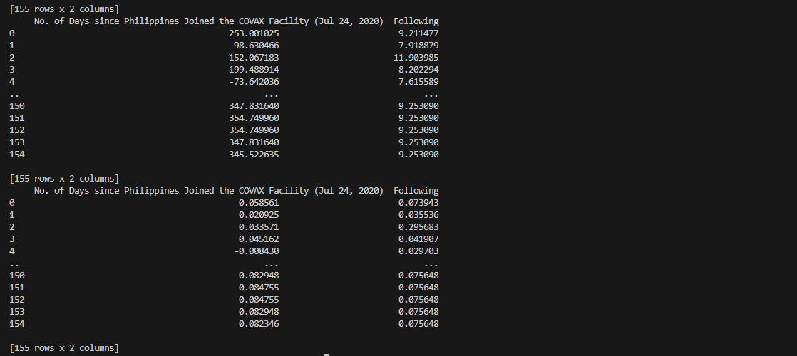
Subsequently, print() can be used to
immediately check that the data points in the aforesaid copies are scaled within the expected ranges and
magnitudes.
Our proposed research question and hypotheses require us to derive
conclusions from the contextual perspective of our gathered tweets. As such, we employ the stage of NLP to
meet this requirement.
The preliminary method was executed by onverting Dataframe to a list
of texts:
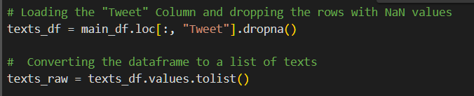
In order to accomplish Natural Language Processing (NLP), the first
step is to convert the dataframe into a list of texts. This is simply done by isolating the “Tweet” column
and dropping the rows with NaN values through .loc() and dropna() methods respectively. And then, we convert the dataframe to a
list using the values() and tolist() methods.
This step is crucial when it comes to preparing the dataset for NLP.
Properly handling the emojis will allow for easier processing of the data and simply removing them from the
text won’t do since they might contain important details about the text.
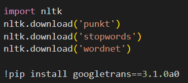
Another vital task before proceeding to NLP is to translate the text to English as it helps us
standardize the format and remove the stopwords from the text which is one of the steps in NLP.
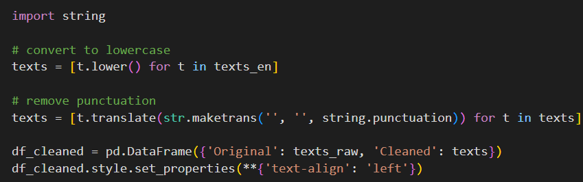
These steps also allow us to standardize the texts and remove
irrelevant characters from them. By doing these, we won’t count the same words twice (i.e. “Data Science” is
the same as “data science”)
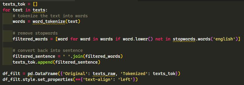
Tokenization transforms the raw texts into smaller chunks of data
that a computer can easily process while removing stop words, which are words that are highly used in the
English language and very insignificant (i.e. pronouns, articles, etc.)
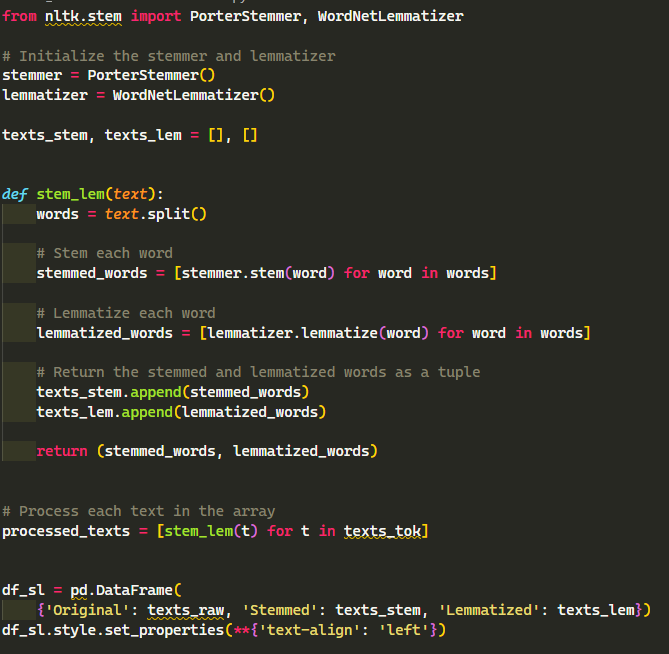
Stemming refers to the process of removing the last few characters of
a word in order to extract the root word. In this way, we can further reduce the number of words to process
given that the word “exploration” will be the same as “explore”.
However, the problem with Stemming is that it will yield inaccurate and unclear results.
Using the same example as earlier, performing stemming results in
“explor”. This is where Lemmatization comes in. Lemmatization is quite similar to Stemming since its goal is
to reduce a given word to its root.